
Motif Discovery Problem
The Motif Discovery Problem (MDP) is one of the most important sequence analysis problems related to discover common patterns, motifs, in DNA sequences. A motif is a nucleic acid sequence pattern that has some biological significance as being DNA binding sites for a regulatory protein, i.e., a transcription factor (TF). TFs regulate the gene expression process by activating or inhibiting the transcription machinery. Understanding this mechanism is a major challenge in biology. A biologically relevant motif must have a certain length, be found in many sequences, and have a high similarity. These three goals are in conflict with each other. In recent years scientists are decoding genomes of many species, increasing the computational workload of the algorithms. Wherefore we need algorithms that are able to deal with these new large DNA instances.
MDP Mathematical Formulation
Given a set of sequences S = { S_i | i = 1,2,...,D } of nucleotides defined on the alphabet B = { A,C,G,T }. S_i = { S_i^j | j = 1,2,...,w_i } is a sequence of nucleotides, where w_i is the sequence width. The set of all the subsequences contained in S is {s_i^{j_i} | i = 1,2,...,D, j_i = 1,2,...,w_i - l + 1 }, where j_i is the binding site of a possible motif instance s_i^j on sequence S_i, and l is the motif length, the first objective to be maximized. To obtain the values of the other two objectives we have to build the Position Indicator Matrix (PIM) A = { A_i | i = 1,2,...,D } of the motif, where A_i = { A_i^j | j = 1,2,...,w_i } is the indicator row vector with respect to a sequence S_i. A_i^j is 1 if the position j in S_i is a binding site, and 0 otherwise. We refer to the number of motif instances as |A| = \sum_{i=1}^D{\sum_{j=1}^{w_i}{A_i^j}}. We also require to find the consensus motif, which is a string abstraction of the motif instances. In this work we consider a single motif instance per sequence. Only those sequences that achieve a motif instance of certain quality with respect to the consensus motif were taken into account when we perform the final motif. This is indicated by the second objective, the support.
Furthermore, S(A) = { S(A)_1,S(A)_2,...,S(A)_{|A|}} is a set of |A| motif instances, where S(A)_i = S(A)_i^1S(A)_i^2...S(A)_i^l is the ith motif instance in |A|. S(A) can also be expanded as (S(A)^1,S(A)^2,...,S(A)^l), where S(A)^j = S(A)_1^jS(A)_2^j...S(A)_{|A|}^j is the list of nucleotides on the jth position in the motif instances.
Then, we build the Position Count Matrix (PCM) N(A) with the numbers of different nucleotide bases on each position of the candidate motifs (A) which have passed the threshold marked by the support. N(A) = { N(A)^1,N(A)^2,...,N(A)^l }, and N(A)^j = { N(A)_b^j | b \in{B} }, where N(A)_b^j = |{ S(A)_i^j | S(A)_i^j = b }|. The dominant nucleotides of each position are normalized in the Position Frequency Matrix (PFM) N = \frac{N(A)}{|A|}. Finally, we calculate the third objective, the similarity, averaging all the dominance values of each PFM column, as is indicated in the following expression:
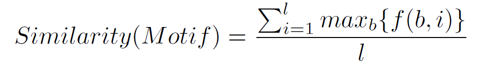
where f(b,i) is the score of nucleotide b in column i in the PFM and max_b{f(b,i)} is the dominance value of the dominant nucleotide in column i.
To guide the pattern search to solutions that have biological relevance, we have incorporated several constraints that should be satisfied by each solution. In motif discovery, motifs are usually very short, so that, finding long motifs means to lose a great computational time. To avoid this, we have restricted the motif length to the range [7,64], where the minimum is 7 and the maximum is 64. In the second objective we have also set a minimum support value of 2 for the motifs of the data sets composed by 4 or less sequences, and of 3 for the other ones (more than 4 sequences). Normally the binding sites are composed by motifs of all or nearly all sequences, and without this constraint is very easy to predict motifs with a high similarity (even 100%) formed, for example, by candidates of only one sequence. Finally, we have applied the complexity concept. The complexity of the candidate motifs should be considered in order to avoid low complexity solutions, for example, the two candidate motifs `AAAA' and `AAAA' are very similar, in fact they are identical, but it is not a meaningful motif. The average complexity for a final motif represents the total complexity score for each candidate motif. We calculate the complexity of a candidate motif by using the following expression:
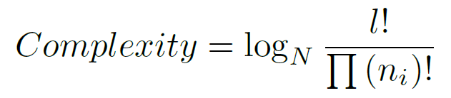
where N = 4 for DNA sequences, l is the motif length, and n_i is the number of nucleotides of type i in {A,C,G,T}. For example, if we consider the motif `AAAA' (n_A=4, n_T=0, n_G=0, and n_C=0) we will obtain a minimum complexity. Otherwise, if we have, for example, the `ACGT' motif (n_A=1, n_T=1, n_G=1, and n_C=1) we will obtain a higher complexity. As we can see in the equation, if we do not normalize the complexities when we compare motifs, the maximum complexity was highly dependent of the motif length. The compositional complexity calculation was revised such that the maximum possible complexity score is calculated for each possible motif length prior to the evolutionary computation. During evolution, each complexity score was rescaled between [0,1] where the maximum possible complexity score was 1. This removed any potential bias in complexity relative to the motif length.
MDP Example
Table 1 illustrates an artificial MDP with motif length = 7. By using the motif instances shown in Table 1a and 1c, we obtain the consensus motif A[GT]TTGAA. Due to there is a tie in the second position of the motif, for this position, we select one of the winner nucleotides randomly, in this case we have chosen the nucleotide T. With this consensus motif, in Table 1d we can calculate the value of the second objective. Those sequences whose motif instances exceed a threshold value of concordance of 50% will be taken into account in the support, in this example we have support = 7. The last step is to build the PCM and the PFM by using the nucleotides of the motif instances that have passed the concordance threshold. Having done that, we can obtain the value of the similarity, applying the equation (1). In this example we obtain similarity = 0.65.
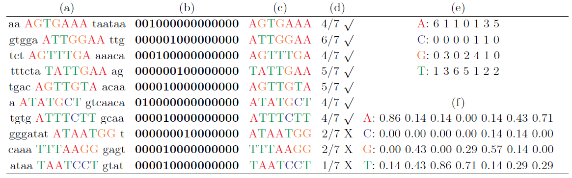
Table. 1. MDP example.
Instances
"i20-0500.fasta" (10.000 nucleotides)
"i20-1000.fasta" (20.000 nucleotides)
"i40-0500.fasta" (20.000 nucleotides)
"i60-0500.fasta" (30.000 nucleotides)
"i20-2000.fasta" (40.000 nucleotides)
"i40-1000.fasta" (40.000 nucleotides)
"i80-0500.fasta" (40.000 nucleotides)
"i60-1000.fasta" (60.000 nucleotides)
"i40-2000.fasta" (80.000 nucleotides)
"i80-1000.fasta" (80.000 nucleotides)
"i60-2000.fasta" (120.000 nucleotides)
"i80-2000.fasta" (160.000 nucleotides)
